 4. Field-effect relationship
4.1 Considerations on the method:
An area in space is the headquarters of a field when it is possible to characterize in it a physical property given by a function of position and time [32]. This definition involves a mensuration process that —for interaction field— implies the acceptance of the existence of an effect on a test object. It is important to notice that for the same field the observed property can be different if the test objects are different. With this restriction in mind and going back to the above-mentioned definition, we might conclude that the field is characterized by its effects, and not by its cause.
What can we say about the method? When referring to the inherent difficulties of the elaboration of electromagnetic field theories, Eisntein commented: "The lack of a systematic method prevented us from getting to a solution." [33]
In my opinion any method to be used in scientific theorization should have the following absolute rules:
1) not to despise confirmed experimental data;
2) not to fill theoretical gaps with controversial experimental concepts;
3) not to defend obsolete theories, regardless of their mathematical elegance and beauty;
4) not to save equations that have proved incompatible with experimentation, although they may appeal to us;
5) to make explicit the goals that theoretical researcher intends to reach in each stage of theorization;
6) to propitiate the necessary revisions of results obtained in previous stages;
7) to propitiate the development of general theories;
8) to propitiate conditions to endow the developed theories with internal coherence;
9) to loathe all and any prejudice;
10) to refuse any bias.
Scientists generally agree, defend and emphasize these rules. Due to unknown reasons, they do not always follow them, as we saw in item 3 of this article.
In field theories, the great step forward was given by Newton. Three hundred years after him, the decisive step is still to be taken, and most theoretical physicists of our century do not believe that such step can be taken. Schrödinger, De Broglie and Einstein are important exceptions to this rule; to quote Popper, for them "scientists should neither abandon the search for universal laws, nor the attempts of explaining any kind of event, starting from its causes." [op. cit. 22].
Actually we know a lot about fields: on what they act, how they act and the consequences of these actions; and we know how to produce them. If we do not take into consideration the paradigms of ignorance, if we guide ourselves strictly by the rules presented above and if we focus the elementary causal agent of the field —something we do miss— we will certainly get to the foundations of a consistent field theory. After this stage and knowing the foundations, we can develop the first phase of the theory, that is, the deductive phase. Starting from this phase and knowing the cause —although hypothetically— we can evaluate its effects thus arriving at the field equations: this is the second phase, or analytic phase of the theory, which will the main theme of this item (4). If the theory is consistent, its equation will reveal a real surprise: "besides the field concept there will be no other concept concerning particles" since we chose to exclude the cause when defining the field.
Let us now analyze the restriction we mentioned at the beginning of this item: the property that characterizes a field can differ if the test objects are different. This inconvenience can and should be avoided. For example, force is not always a good property to characterize a force field: its value only became a position function when refers to the same test object. In the case of electric field the artifice adopted by the classic theory is simple: E property is defined as the force per electric charge unit
|
E = F / q, | (4.1 ) |
in which q is given by Coloumb’s law.
The artifice will be exclusively efficient if all the elements which are sensitive to the field can be imagined as one of the loaded spheres used in Coulomb’s experiment. A particle not presenting such property, i.e., that cannot be thought of as an electric charge, will present an anomalous behavior in the field under consideration. This anomaly is provoked by the bad characterization of the field rather than by properties inherent to the particle (hidden variables). There were countless experiments in this century trying to show an anomalous behavior of electrons when submitted to fields characterized by the 4.1 expression; and a collection of these anomalies can be found in any modern physics textbook.
There are, however, some very uncommon conditions under which the electron simulates a classic behavior, as if it really possessed a q electric charge; and this will be the clue we are going to use together with 1 to 4 hypotheses in order to get into the mysterious world the elementary particles. We shall interpret these rare experimental occurrences, trying to establish a background so that we may get to the electron equation foreseen in hypothesis 3.
4.2 The field of electric effects:
Through different methods Thomson (1987) and Milikan (1910) realized that the electron in a uniform electric field behaves in a similar way to an electric charge with a spherical symmetry. This similarity induces us to consider the uniform electric field as the ideal place to star our analysis.
Let us imagine a conductive sphere with a long radius and electrically loaded. The electric charge thus imagined produces a practically uniform E Coulomb’s field: it is enough to restrict the domain of the field to small volumes with the longer axis practically non-existent in relationship to the radius of the sphere. The adopted reasoning similar to the one we employ when the gravitational field near the earth is practically uniform.
In this sphere the electrons are distributed as it is established by Corollary 4: with its main axis perpendicular to the S spherical surface. As the radius of the sphere is quite long, we can represent the electrons as in Figure 6.
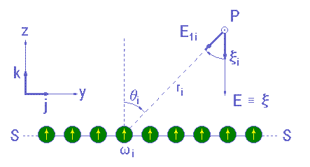
Figure 6: Comments in the text.
On a generic point P = (x, y, z) in the domain of E field, observing the Superposition Principle it is possible to equate E in this way:
|
|
(4.2) |
Ei being the contribution of the electron i to the E field on point P.
One of the possible solutions for the 4.2 equation for Ei of the i electron is given by Coulomb's equation:
Solution 1 (E i1): |
|
(4.3) |
in which K is a proportionality constant related to the definition of an electric field. As we have seen, this solution proved incompatible with many of the experiences made in the 20th century.
Another solution —also compatible with Coulomb’s law in terms of electric charges— is:
|
Solution 2 (Ei2 ou x i): |
(4.4) |
with θi shown in Figure 6. x will be called electric effects field in order to distinguished from the classic E, which will go on being called electric field. In the present discussion we have: x = S xi = E.
We shall now demonstrate —in a more convincing way— that solution 2 (equation 4.4) is actually compatible with Coulomb’s law.
4.2.1 The x field of a loaded conductive sphere:
From corollary 4 and equation 4.4 we conclude that the xi electric effects field of an electron belonging to an infinitesimal surface ds of a loaded spherical conductor will be:
|
|
(4.5) |
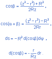
The meaning of the variables found in equation 4.5 can be obtained from the exam of Figure 7;
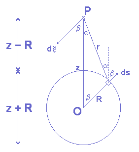
Figure 7: Comments in the text
dn indicates the number of electrons contained in ds. Under these conditions, the electric effects field in P —due to ds— will be:
|
|
(4.6) |
and N = 4pR² dn/ds is the total number of electrons composing the electric charge under consideration.
It elapses from the symmetry of the problem:
|
|
(4.7) |
and from equation 4.6:
|
|
(4.8) |
With the aid of figure 7 and calling the azimuthal angle φ, we can establish the following relationships:
 |
(4.9) |
Substituting 4.9 in 4.8 and simplifying, we have
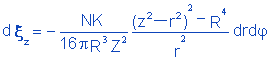 |
(4.10) |
Integrating 4.10 [z > r and z < R] and observing 4.7, we have:
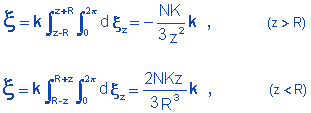
Using the conventional notation for distances (r = distance from P to the center of the sphere = z) we finally get to:
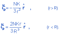 |
(4.11) |
4.3 The electrostatic force
When we think of x (electric effects field) as a force field, we should keep in mind that, generally speaking, after the action of x is calculated by trivial methods, it leads us to the force acting on an electron and not on an electric charge. It is also important to observe that the x field of an electron (equation 4.4) is neither of Coulombian nor Gaussian type (the field lines do not begin and finish in the electron). Nevertheless, the x field of a spherical electric charge (equation 4.11) is a Coulomb’s field in its exterior..
A negative test charge q placed in a uniform x electric field and balanced by its weight will be subject to an electric force F with F = S Fiq. Here Fiq is the force exerted by a generic electron i on the electric charge q, as shown in Figure 8.
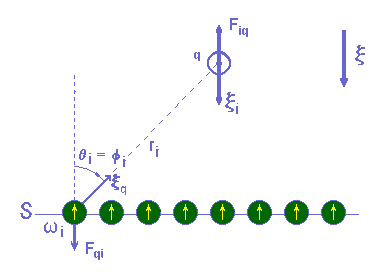
Figure 8:
Comments in the text
The modulus of F is proportional to the modulus of the x field, or
F = C1x
and thanks to the Superposition Principle —valid for forces acting on Coulombian charges— we can also write:
| Fiq = C1xi . | (4.12) |
The electric effects field xq produced by the charge q is of the Gaussian type and also of the Coulombian type, according to equation 4.11 for r > R. If xq is not very intense in relationship to x, we can despise the inductive effects. Joining the appropriate proportionality relationships, we obtain:
|
4.12: |
Fiq = C1
xi |
|
| 4.4: |
xi
= C2cosθi
/ri2 |
(4.13) |
| Coulomb law: |
xq
= C3/ri2 |
in which C1, C2 and C3 are constant. Solving the system of equations 4.13 for Fiq, we have:
Fiq = C4 xqcosθi
or, in vectorial notation:
Fiq = C4 xqcosθi k .
The surface S will be subject to the reaction - F = S Fiq. It seems reasonable to expect that Fqi = - Fiq (individualized action and reaction [34]). If we accept this equality, we will get to the expression:
Fqi = - C4xqcosθik .
It will be convenient to use f to refer to the angle between the w vector electron and the direction of the field to which the electron is submitted. In the specific case under consideration (figure 8) —and because the electric field xq is Coulombian— this angle equals θ, defined through the equation 4.4 (fi = θi). So the previous equation can be written as:
Fqi = - C4xqcosfik .
To generalize, we will say that the electrostatic force acting upon an electron placed in an electric field x, can be expressed as:
|
F = Cxcosfv |
(4.14) |
with f = the angle between x and v.
4.3.1 Electrostatic force between loaded conductive spheres:
Let us suppose that we have x, denoting an electric field function produced by a loaded conductive sphere, with center in P = (0,0,0) point, plus an electron of the infinitesimal surface ds of another loaded conductive sphere placed in a Q = (x,0,0) point. This electron will be subject to an electric force F, given by 4.14, which —according to Figure 9— will be:

Figure 9: Comments in the text
|
(4.15) |
The inductive effects were despised in a similar way to the dodge adopted in the analytic study of Coloumb’s law. This implies considering the electrons as fixed and restricted to a centrifugal direction. The force on ds will be, then:
|
(4.16) |
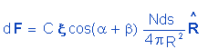
The dFy and dFz components are canceled in pairs. Therefore,
|
(4.17) |
With the aid of figure 9 we get to the following relationships:
|
(4.18) |
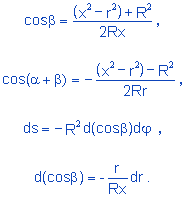
Substituting 4.18 in 4.16 and observing the value of x given by 4.11 for r > R, we obtain:
|
(4.19) |
The expression 4.19 is nothing but Coulomb's law, expressed in terms of the numbers of electrons N and N' contained in the considered Q and Q' charges.
 |
Contents |  |
| Return | Advance |